Haplotype Diversity in Africa
Introduction
At Bixbio we work with the most diverse genomic data, all of the time, and we believe that diversity is the most important differentiator in both genetic research and its practical applications. So one might expect that we’d be very good at explaining why we care about genetic diversity, and even more fundamentally, what genetic diversity is. But the truth is that genetic diversity isn’t just one simple concept, which means that it’s often talked about in ways that might not make intuitive sense, using broad strokes or somewhat opaque statistics. A proper explanation requires a small amount of patience – and a decent amount of good-quality data.
The goal of this post is to attempt to provide such an explanation for a general audience, highlighting the importance of African data along the way. The two are almost inseparable after all, given that Africa “harbours more genetic diversity” than any other continent [1]. Here we’ll try to unpack what that means.
We start with a basic description of genetic variation and the mechanisms that give rise to genetic diversity, along with a useful illustration of global diversity from an African perspective. The remainder of the article then works towards a more complete demonstration of genetic diversity by describing how it originates at the haplotype level. If you already know what a haplotype block is1 you might choose to skip straight to the end, perhaps skimming the figures along the way.
This topic lies at the heart of what we do at Bixbio: developing tools to analyse diverse genomic data as accurately and powerfully as possible. Much of that work is statistical in nature (I am a mathematician and computer scientist by training), and the content of this article reflects this. So it’s worth mentioning that although an effort has been made to be clear and thorough when explaining any biological concepts, the primary intention here is not to provide a complete lesson in human or population genetics – for that one should probably find a good textbook.
The basics
Starting at the beginning: each of us inherits 23 chromosomes from each of our parents, giving us 23 pairs of chromosomes, one of which is a pair of sex chromosomes – XX or XY. The genome refers to an individual’s complete set of DNA, made up of their chromosomes and a small amount of mitochondrial DNA inherited from their mother. DNA is made up of four nucleotides (represented by As, Cs, Gs, and Ts), and the ‘length’ of the human genome measured in nucleotides is around 6.2 billion base-pairs (bp) – about 3.1 billion bp per set of chromosomes.
If you consider any two individuals, the vast majority of their genomes will be the same – they’ll have about 99.9% of their DNA in common. But this doesn’t mean that 99.9% of the human genome is fixed, or common to everyone. Rather, there are millions of positions along the genome where variation can occur, and this variation can take different forms: it could involve a change to a single nucleotide (so-called single-nucleotide variants, or SNVs); sequences in which a few nucleotides are ‘inserted’ or ‘deleted’ relative to one another (indels); or large-scale differences in the DNA sequence (structural variants, commonly defined as involving more than 50 bp). Generally, about 80% of the differences between two genomes are SNVs.
Regardless of length, the known possibilities at any given position are referred to as alleles. Most variant positions will only have two possible alleles, and one allele (the ‘major’ allele) will often be far more common than the others. For the sake of illustration, a hypothetical pair of sequences involving a single-nucleotide variant might look something like the following: AATTT and ACTTT. In this case the variant’s alleles are A and C. Sequences implying an indel might be GTGTGT and GTGTGTGT, in which case the alleles could be defined as T and TGT.
Since each of us has two ‘copies’ of each non-sex chromosome, we also have two alleles at each position where variation is known to occur. Once DNA has been sequenced (hardware) and analysed (software), we end up with what are known as variant calls: records that give the likelihood of a genome containing a variant allele on one or both strands of DNA – known as heterozygosity and homozygosity respectively. One of the difficulties when using short-read DNA sequencing (the most common technology) is that it is in general not possible to ‘phase’ alleles across positions, separating alleles of the maternal chromosome from those of the paternal one, and thereby reconstructing the individual chromosomes.2 This is not a critical issue, since a lot of genomic analysis occurs at the single-variant level, but it will be important in understanding later sections of this article. It explains too why so many statistics in genomics are currently expressed in terms of simple variant counts, even though variants are not the most natural way to think about genetic diversity; and doing so can, at times (or without proper context), be somewhat confusing.
Population groups
Given two individual genomes then, the ‘99.9% similar’ statistic stated above comes from the fact that the first will differ from the second by about 5–7 million alleles. We say 5 to 7 million because it depends very much on who the two individuals are. And this is where things get interesting.
The 1000 Genomes Project [3], or 1KGP, is one of the most important datasets in genomics. And like all other genomic datasets, databases, and biobanks, it stratifies its data at multiple levels. The most important of these is ethnicity, i.e., ethno-linguistic groups such as Han Chinese, Gujarati Indian, Toscani Italian, etc. The 1KGP dataset is an incredible achievement and resource, but when viewed at this level it is clear that it represents only a small slice of global genetics: its 26 ethnicities from 21 countries account for just a fraction of all of human diversity.
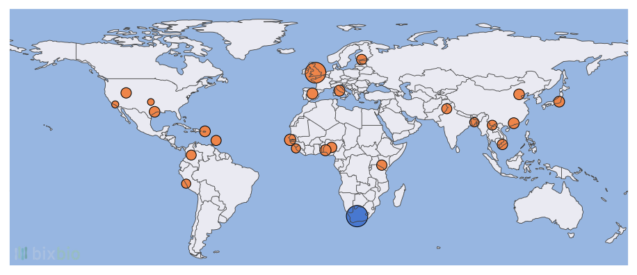
The 1KGP data is often grouped at higher levels as well, for instance into five continental regions: Sub-Saharan Africa, Latin America, Eastern Asia, Southern Asia, and Europe. The difficulty with such groupings is immediately apparent: what about Northern Africa, the Middle East, etc.? Which parts of Europe are represented? (Britain, Finland, Spain, and Italy.) Does Sub-Saharan Africa include Southern Africa? (No.)
And more importantly, does it even make sense to talk about different ‘groups’ of humans? The answer to this is both yes and no: yes, because if two groups of people don’t cross paths for long periods of time their genetics will reflect this – we will be able to predict which group an individual belongs to by looking at inherited patterns in their genome. And no, because human genetics exists as a spectrum [4]. The fact that it often looks as though it can be partitioned into neat categories is due to the difficulty of collecting genomic data – of course sampled individuals from Western Africa and Eastern Asia will have noticeably different ancestry. But for every two seemingly distinguishable groups of people, we’ll almost certainly be able to find a group that lies in between and bridges the genetic gap. This is not to say that there is a problem with the 1KGP or any other dataset, but simply a reminder that those of us who make use of such datasets have a responsibility to represent them with fidelity.
Disclaimer aside, the truth is that continental groupings are useful for genetic analyses, since they are naturally intertwined with the migrations of ancient human populations, and therefore with human evolution and genetic diversity. In what ways do we see this? Well for one (returning to the example above): the genomes of two individuals sampled from Europe, Asia, or the Americas will differ by roughly 5 million alleles across perhaps 4.5 million variant positions. This is the case if the individuals are of the same ethnicity (but not close relatives), or if they come from opposite ends of the world. If one (or both) of those individuals were from Africa, however, the difference would be significantly greater: around 6.5 million alleles across 5.5 million positions. Two individuals from, say, a Zulu population in South Africa will have at least 6 million allelic differences – as will a Zulu and Luhya (Kenyan) pair, and a Zulu and Dai (Chinese) pair, and a Luhya and Toscani (Italian) pair. If neither individual is of African ancestry, however, there will be about 20% less genetic variation: between two Toscani individuals, say, or Toscani and Finnish, Finnish and Gujarati (Indian), etc.3
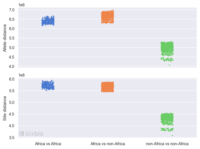
The bottom line is that in general, two people from anywhere outside of Africa are more genetically similar to each other than two people from within Africa. And furthermore, diversity on the African continent can be seen as the norm, since the level of similarity between two African individuals and between an African and a non-African is roughly the same. At Bixbio we sometimes express this remarkable fact by saying that from an African perspective, everyone is African.
Mutation and recombination
How is it that genomes differ in the first place, and to such varying extents? We’ll continue to explore this in the following sections, but the brief answer is that there are two mechanisms at work: random mutation, which introduces new alleles into a DNA sequence, and recombination, which mixes existing chromosomes to create new, hybrid ones. Mutations are the ultimate source of new genetic variation (and diversity), but the way in which they are propagated throughout a population is due to recombination.
Consider again the fact that you have two copies of each chromosome, but that your child only inherits one from you – which one do they get? The marvellous reality is that chromosomes are inherited in a ‘patchwork’ manner: the chromosome 1 that you pass on to your child,4 for example, is created when your two copies of that chromosome come together and exchange stretches of DNA during recombination, as part of a process called meiosis. So each stretch of the chromosome you received from your father matches one of his two copies of that chromosome: one such segment may match the one from his father, while a stretch of DNA further along the same chromosome might match the one from his mother. This means that although your DNA is for all intents and purposes half from your mother and half from your father, it is not necessarily a quarter from each of your grandparents.
Both mutation and recombination occur randomly, but recombination is more likely to occur at certain ‘hotspots’ throughout the genome [5]. Together the two mechanisms ensure that the DNA of every sperm or egg cell is essentially unique. The former might take place on the order of 100 times across the genome, and the latter perhaps once or twice per chromosome [6].
Over thousands of generations, the ancestral tree of any population group will become incredibly complex,5 but certain ancestries (and ancestors) will come to dominate the group’s genetics at certain times. Two seemingly contradictory characteristics will arise: on the one hand, the genome of any given individual will contain DNA from essentially all of these ancestries, since they will have mingled and recombined over time. But on the other hand, at the smaller scale – where the DNA has mostly been spared the shuffling effect of recombination – the ancestral genomes will still be intact and distinguishable, along with the mutations that accumulated and differentiated them in the first place.
On the far more comprehensible time scale of our own lifetimes, this means that although none of us shares a complete genome with anyone else (apart from identical twins), we all share many small segments of DNA with people all over the world – and the set of people we have DNA in common with differs per segment. We are, each one of us, a human mosaic. Because of recombination, the genetic history of a population is imprinted on the genomes of all of its members, not siloed into distinct subgroups. This remarkable fact, you might have realised, means that each of us carries a trace of the history of the human race in our DNA. We just won’t be able to make sense of it without comparing it to the DNA of others.
The DNA segments mentioned above – the ones shared by many people across a population, or across the world if they are old enough – are the building blocks of genetic diversity. Accordingly, they are called haplotype blocks, or haploblocks for short. Stated another way, a haplotype block is “a region of the genome with a shared pattern of ancestry” [2]. The simple fact is, as we will see below, that non-African populations have significantly fewer distinct haploblocks than African populations, consistent with the consensus that all of these populations at some point migrated out of Africa, and by doing so underwent evolutionary ‘bottleneck’ events.
The statistics
Rewinding slightly before we look at examples of haploblock variation, it’s worth reiterating that the majority of computational genetics currently doesn’t deal with haplotypes.6 Plenty of analysis is done at the individual variant level due to the mechanical, statistical, and computational difficulty of inferring and working with haplotypes. This leads us back to our statistics: how else do the variants in a dataset reflect the underlying diversity?
One of the most commonly presented statistics used to describe diversity is the number of distinct alleles observed (or ‘discovered’) in a sample population. Variant alleles that have never been seen before are termed novel, and are generally used to support the uniqueness or importance of new genomic data. More interesting than alleles that are only found in certain datasets, from our perspective, are those that are found in specific subpopulations. For instance, considering just the 1KGP dataset so as not to inflate the number of African samples, we might report the following statistics based on its 2,504 whole-genome samples:
- The total number of (distinct) alleles observed in the dataset: about 272 million alleles across 136 million variant sites (including reference – GRCh38 – alleles). This is influenced by both the size and diversity of the dataset.
- The fraction of the total allele set found in specific subsets of the data – for instance based on continental regions. If only the 661 African samples had been sequenced, 49% of the distinct non-reference alleles would have been observed, compared to 29% if only the 503 European samples had been collected. There were 66 million such alleles present in the African subset, compared to 39 million in the European, and 102 million in the combined non-African subset of the data (1,843 samples).
- The number of alleles that are unique to subsets of the data: there are 33 million alleles that are only observed in the African subset of the data, for example, compared to 18 million alleles unique to Southern Asia.
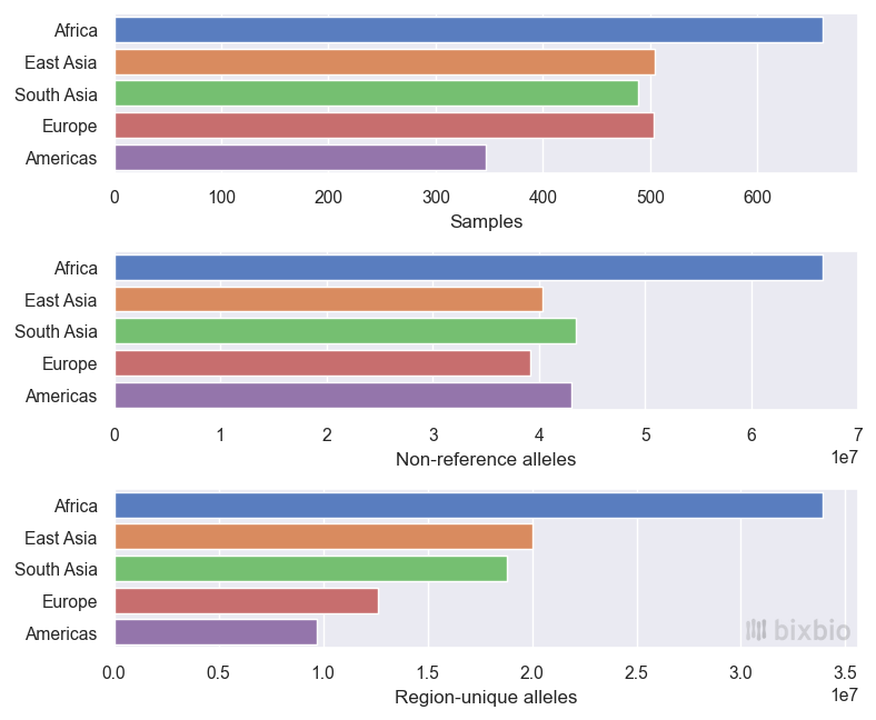
One can of course go further than this as well: it’s sometimes useful to see the rate at which distinct variants are discovered in a certain dataset, for instance by plotting the number of alleles observed in a sample of 10 individuals, then 50, 100, etc. One would see that genomic data from African ancestries yields more alleles with fewer samples – i.e., at a faster rate. It’s worth noting here though that the majority of genetic (minor) alleles are rare; that is, they only occur in a very small proportion of a population. This means that the rate at which new alleles are discovered decreases as more samples are sequenced.
These variant/allele statistics make it perfectly clear that African genetics is significantly more diverse than that of any other continent. And for practising researchers these numbers are the important ones – they directly quantify diversity based on the data we get from sequenced DNA. But consider them in isolation: do they make intuitive sense? Do they lead to more questions? For instance, are variant alleles randomly occurring in Africa at a greater rate than elsewhere? (No.) Why are there significant numbers of alleles that are unique to any region, not just Africa? (The accumulation of random mutations through either chance or selection.)
And then reflect back on the pairwise statistic we introduced earlier: how can it be possible for subpopulations to have so many unique genetic variants, and at the same time for the number of differences between two individuals from that group, or from two groups on different sides of the world, to be roughly the same?
The simple explanation
This explanation has of course been anything but simple so far, but as with most science7 its individual pieces are relatively easy to grasp, and understanding the concept as a whole mostly involves placing the pieces in logical order. So let’s recap:
- Our genomes are made up of 23 pairs of chromosomes (plus some mitochondrial DNA).
- Each individual chromosome is inherited from one of your parents, and is a unique (re)combination of your grandparents’ chromosomes along with a small amount of random variation.
- Over many generations, ancestral genomes will spread throughout the population as small segments, meaning that your DNA is made up of stretches that are shared with many other people. These stretches of DNA are haplotype blocks, and they can theoretically be used to give a high-level description of all of the possible genomes in the population.
- Haplotype blocks are also the vehicles of genetic diversity: they represent the different forms that a certain region of DNA can take, and the number of possible haplotypes is directly coupled with the level of diversity in a population.
How does this explain the difference between African and non-African genetics at the statistical level? As a group of people separates from a population, it takes with it only those haplotypes present in the group, and any new variation added to the two groups’ genetic pools is no longer shared between them. Note also that recombinations between similar haplotypes don’t serve to deepen diversity in the way that diverse recombinations do. This is the case with populations outside of Africa: they have fewer distinct haplotypes, and a relatively small amount of variation of their own. (The theorised out-of-Africa migrations [7] didn’t take place that long ago on the anthropological timescale after all.) These populations all exhibit a similar subset of the haplotype variation still present in Africa, and as such they are less genetically diverse than African populations. This essentially answers the two main questions posed above, namely:
Why do genome comparisons involving African individuals yield more allelic differences? One can imagine comparing small blocks of the genomes separately: if either of the genomes come from a population with significantly more possible haplotypes (as is the case in Africa), there is a smaller chance of the haplotypes (and alleles) matching.
Why do non-African populations appear similar in spite of their unique variants? Population-specific variants do differentiate global populations, but their effect is slight when compared to the differences due to ancient haplotype diversity. On an evolutionary timescale, we (human beings) have spent far more time acquiring shared variation in Africa than we have acquiring unique variation outside of Africa.
The example
The goal of this article (if you recall) was to demonstrate the difference in genetic diversity inside and outside of Africa, and as we just mentioned above, haplotype blocks are well suited to doing so. So consider a certain section of the human genome: the gene CYP2D6. This gene refers to a region of about 6,000 bp on chromosome 22, roughly 80% of the way along its 50-million bp length. The CYP2D6 gene is of particular interest in genomics because the enzyme it encodes is involved in the metabolism of about 25% of commonly prescribed drugs [8]. For the sake of this article it is of no special interest – we could have chosen any region of the genome – but it is worth mentioning that protein-coding regions such as these are thought to be less diverse than the remainder (and majority) of the genome.
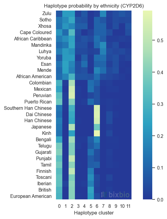
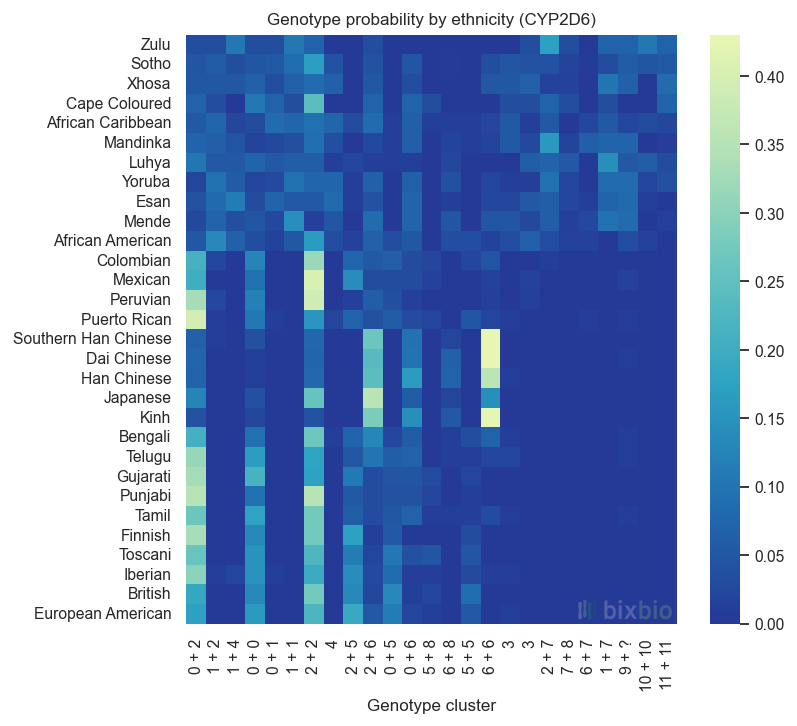
The following visualisations are based on the combined 1KGP/Bixbio dataset of 2,816 individuals. From this data there are 377 observed positions along CYP2D6 where variation occurs, and 377 alleles in total. Of the non-major alleles at these sites, most are infrequent: only 44 occur in more than 1% of the dataset. By clustering the variant call patterns of individual samples, we see a few common genotypes: that is, variant calls for both chromosomes for each individual. With a further round of analysis we can then recover the individual haplotypes in each genotype cluster by noting that the alleles observed in each genotype are the union of the two underlying haplotypes’ alleles, and that the true set of haplotypes must ‘sum’ to the genotypes. It’s important to note that, like all statistical inference, this is an approximate process – although in this case the data is relatively easy to make sense of.
In the end this approach identifies a total of 12 haplotype clusters in the 5,632 genomes in the data set, across 30 ethnicities. Each haplotype is defined by 6 alleles on average. This of course does not mean that all of the individuals treated as possessing a given copy of CYP2D6 have exactly the same sequence of that gene – the clustering process likely ignores spurious differences such as sequencing errors or very recent mutation – but it is immediately apparent which ancestral ‘version’ of CYP2D6 each individual has.
Figure 4 shows the fraction of each ethnicity’s samples in a given haplotype group (so each row sums to 1). This figure summarises many of the points we’ve made in this article, and hopefully now does so in a more intuitive way than the statistics of previous sections. We see, as expected, that significantly more haplotypes – i.e., versions of the gene – exist in African subpopulations than anywhere else, and that non-African variation is by and large a subset of African variation. The non-African subpopulations share strikingly similar sets of haplotypes, with some divergence in Eastern Asian ethnicities. Compare this figure to Figure 3: it should now be clear why Africa has more distinct alleles in total, as well as many alleles not found in any other region (presumably from haplotypes unique to Africa).
The genotypes present in the dataset can be visualised in the same way, demonstrating how haplotypes might be paired together in different subpopulations. These genotype clusters essentially describe all of the possible versions of CYP2D6 that an individual might have (based on the small sample of healthy individuals in the dataset). We see 25 such clusters,8 showing similar patterns to that of the previous figure but slightly obscuring the fact that many genotypes overlap due to shared haplotypes.
The point
There are essentially three main points here:
- Firstly, that we all share a common human ancestry, as told by our DNA. Each of our genomes is a unique combination of haplotypes, but these haplotypes do not ‘belong’ to us – they are shared with many others in the population. Human genetics is dense, complex, and exists as a spectrum, but at the small scale it can still be understood and represented relatively easily.
- Secondly, Africa is home to significantly more genetic diversity than anywhere else in the world, and the genetic diversity found elsewhere is essentially a subset of Africa’s. One way to make sense of this is simply to understand that for any region in the genome, the number of distinct haplotypes found in Africa is greater than the number found anywhere else; as ancient people groups migrated out of Africa, they took with them only a subset of African haplotype diversity.
- And thirdly, diversity matters. To understand global genomics, we need to understand genetic diversity, and to understand diversity we need to understand African genetics.
This third point is one that we haven’t touched on directly yet, but as a company it forms the core of our vision. Genomic medicine is already relatively commonplace in developed countries, and it will only become more so – in all likelihood quite rapidly. Its applications are varied: a genome might be sequenced in an effort to screen for certain diseases, to diagnose certain genetic conditions, or to predict the risk of a specific individual developing a disease [9]. On the treatment side, the field of pharmacogenomics studies the impact that genetics has on the safety and efficacy of drugs, and involves tailoring treatment plans to an individual based on their DNA – for instance by predicting which drugs will work best. Gene therapy goes even further, by inserting healthy versions of a gene into a patient’s cells [10].
All of this work relies on sophisticated biological and statistical analyses, since one needs to find associations between genomic features and disease mechanisms. Because of this, modern drug development is now highly dependent on such data. The catch, however – and the reason that articles such as this one, and companies such as Bixbio, are necessary – is that global populations are not equally represented when it comes to such research. Far from it. The most common form of analyses used to look for genetic markers correlated with disease – genome-wide association studies (GWAS) – are heavily skewed towards European data: at the time of writing only 0.2% of all GWAS participant data is estimated to be of African ancestry [GWAS Diversity Monitor, 11]. This means that predictions and treatments don’t necessarily work as well (or at the very least aren’t as well understood) in non-European populations. In light of the examples above, what comes to mind when you hear this? Does it seem… sensible? How much knowledge, and how many advancements, are we missing out on?
There are, thankfully, promising efforts to address this imbalance: many public genomic datasets place a high priority on collecting samples from under-represented population groups; graph reference genomes have arisen as a means of reducing the bias introduced by current, linear reference genomes; and valuable research is being done to support the effective presentation and analysis of multi-ancestry genomic data. (See for instance the HPRC, or gnomAD). But the problem does still remain – and at least in the case of GWAS is only getting worse – due to the fact that almost all DNA sequencing takes place in developed countries.
Our hope, and goal, is that current efforts to diversify genomic research will gain traction and be able to transform the field, since if one thing is clear it’s that those working in it desire a society in which all individuals have access to genomic medicine of the same quality. And something that should hopefully also be clear by now is that human genetics is a fascinating, inspiring field to work in: our genetic history is simultaneously incredibly diverse and surprisingly transparent. Perhaps if it was more widely understood, all genetic research would start where that shared history does: here in Africa.
Acknowledgements
The input of a few colleagues has been invaluable both in performing the analysis outlined here and in discussing and editing the article: thank you to the Bixbio team – James Ross, Tyronne McCrindle, and Pieter Ross – as well as to Jon Ambler9 and Caroline Foden10 for all of their help.
References
Footnotes
This is simply due to the fact that the DNA is sequenced as small ‘reads’ that must then be pieced together, and two positions have to be spanned by a single read for their alleles to be phased. There are statistical approaches to solving this problem. Newer, long-read technology also addresses this issue, but has shortcomings of its own.↩︎
There will of course be populations that exist in between these two extremes, as mentioned above. But in general this stark difference holds.↩︎
The non-sex chromosomes are numbered from 1 to 22.↩︎
And ‘tree’ is actually a misnomer here, since you are related to anyone else via many different paths of possibly very different lengths. These paths can also merge or split in ways that a tree structure wouldn’t: e.g., you’re related to your maternal cousin via your grandmother, but also via a much longer route through your father and another common ancestor.↩︎
A haplotype, in this context, is a stretch of an individual’s genome that has been resolved and determined to come from a single copy of one of their chromosomes, i.e., a set of variants that have been inherited together. The term ‘haplotype block’ refers to the shared inheritance of such a region within a population.↩︎
Quantum physics aside.↩︎
How many would you have expected to see? Given 12 distinct haplotypes, there are in theory 144 possible pairings.↩︎
At the Institute of Cellular and Molecular Medicine, University of Pretoria.↩︎